Experimentation

Multiplexer Representation Test

In the preceding chapter, I have shown how the XCS system learns the 6-multiplexer problem. I want to show here that this learning ability is a property that holds for this problem because of the regularities that are compatible with the XCS system's representation and generalization functionality (that I associate with information compression). In the general case of a problem that is not well understood and that must be solved, applying a particular algorithm will help to understand the functionality and limits of the algorithm, as well as the properties of the problem. I intend to show by a trivial example that the representation of a problem plays a fundamental role for adaptive behaviors and will relate this to the question of information compression.

The Multiplexer Description

I have described previously why the multiplexer is used as a test case for the XCS system. The multiplexer function is a boolean function, which is naturally suited for learning by the use of classifiers; its standard description is based on the use of an address set indexing a value set that allows generalization to occur on individual bits as patterns of zeroes and ones with wildcards. The term ``description'' that I use here should be understood as the symbolic representation of input signals. The internal symbols used by classifier systems as messages are strings of bits and the natural symbol associated with an input signal is the bit string of the signal itself, but other problems do not necessarily have such a ``natural'' mapping of inputs onto internal symbols.

For the multiplexer problems, the natural description is based on the use that is made of the function by humans, but actually, the description depends on perception of the problem by the system. And the actual problem to solve is of distinguishing inputs into two categories, those that are mapped to a one and those that are mapped to a zero. The regularities of the function are simply regularities of the description of this function. In the multiplexer case, we use a description that is known to be expressive simply because it is the one we use as humans to understand the problem and associate an additional meaning to the order of the bits and their signification. This proves to be a good description for a classifier system to learn.

In the general case of a misunderstood problem, there is no guarantee that the classifier system would obtain descriptions that are compatible with its internal adaptation mechanisms. Imagine, for example, that the multiplexer problem is described as a random permutation of the input signals and that the XCS must learn this new mapping. There will be no reason for it to be able to make good generalizations if these permutations do not offer some degree of compatible regularities (i.e. regularities over single bits in the description).

Regularities in the Description Space

By looking more attentively at the XCS classifier system applied to this problem, there being only two levels of reward implied by the input messages, the information content of an input message is only one bit of information, distinguishing the reward options available to the system when it chooses an action. The role of the algorithm is thus to extract this information and use it to make a decision about the amount of reward it has been programmed to choose. 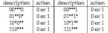To this aim, the generalization mechanism of the XCS system finds a minimum of sixteen general classifiers that resume this decision policy, the classifiers shown on table 8.1. For each general condition, the classifiers that advocate actions zero or one are accurate. Obviously, this representation of the problem used is suboptimal, since the only information content of an input string is one bit, but it still is very close to an optimal representation.

  

Figure 8.1: Complete family of 16 accurate maximally general classifiers.

To illustrate the generalization capability of the XCS system, I have used various permutations of the natural representation of the problem and applied the classifier system to these new problems. In order to give a quantitative measure of the distance between the original description and the permutation over this basic description, five types of permutations have been used. The permutations are of order 2 to 6, meaning that in permutations of order n, n interactions between bits of the original description can be introduced (interactions in a sense that can be related to the epistatic interactions as studied by Kaufmann in [28]). The permutations are constructed in the following way: n bits of the original representation are swapped, then a random permutation over the n-dimensional space of the selected bits is operated. As a result, the larger the n, the further the descriptions provided to the classifier system are from the original. When n=6, any function of $\{0,1\}^6 \longrightarrow \{0,1\}$ can be reached. Additionally, the permutation leading to an optimal representation for the classifier system has been used as a reference for the learning curves of the system. This permutation can be obtained by mapping subspaces of the input space onto a permuted description as described on table 8.2.

  

Figure 8.2: An optimal permutation of the input signal.

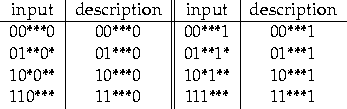The inputs that match input patterns on the table are mapped to the description patterns in the following column of the table. The unspecified bits can be mapped to any other unspecified bit position. For this permutation, all the information content of the input that must be used to obtain a reward or not is contained in the last bit of the description strings, so that the classifier system can build a complete and accurate family of classifiers with only four general classifiers in its population, those with conditions *****0 or *****1 and actions 0 or 1. Other descriptions are optimal in this sense, but due to the genetic search algorithm used to find new classifiers, classifiers with longer defining lengths are slightly suboptimal for crossover operations (defining length is the distance between two specified positions in a pattern, for example the pattern 01*00* has a defining length of 4 and the pattern *0100* a defining length of 3).

For the experiments, one must be aware of the fact that the space of all possible inputs to a function over $\{0,1\}^6$ has 2⁶=64different elements. Learning to map all the inputs correctly for a reward function with just two levels requires twice that number of specific classifiers or 128, when no generalization is used (cf. tabular Q-Learning). For this problem, there are 3⁶*2=1458different classifiers (including the general classifiers) available to the system and, depending on the regularities in the function to be learned, the minimal amount of classifiers needed to accurately learn the function range between 128 in the worst case and 4 in the best case. Therefore, whichever function the XCS must learn, if it is allowed to have a population of more than 128 classifiers, it could learn the function by using only specific classifiers. On the other hand, if less that 128 classifiers are allowed in its population, the function must have regularities that are compatible with the generalization mechanism of the classifiers system, if the system is to learn it correctly.

Result Plots

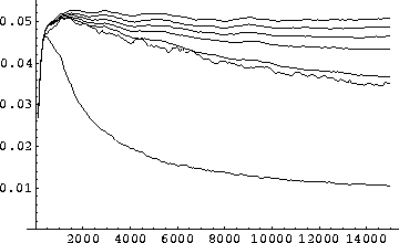
In the figures 8.3 to 8.5, I illustrate the learning curves obtained for each order of permutation, when the classifier population size allowed in the system is 400. The various curves show that with more interactions in between the bits of the problem description, the learning ability of the classifier system is reduced. In the optimal case where only one bit sums up all the information about the function, the classifier system quickly reaches 100% performance. The population diversity then slowly reduces down to 25 individuals as the unnecessary classifiers are eliminated by the genetic algorithm. The normal case is then only slightly better than the learning of functions with order two permutations from the normal description and we can see that each increased permutation level introduces a degradation of the learning ability of the system. Although this degradation is apparent, the system still exhibits a good learning ability for these problems and the prediction curves are still on a slight increase at the 10,000th step. On the population curves, one sees that in each case, the classifier system first generates a wide variety of classifiers, until the 400 individuals limit is reached at 1300 steps. These individuals are then evaluated and after the initial evaluation phase, the inaccurate classifiers start to be eliminated from the population and the overall population diversity gradually reduces to a minimal amount of distinct types of classifiers. Except for the optimal description case, the increase in population continues until about the 2000th step, where it reaches its peak (the overall population is now 400). In the optimal case, the elimination process is intense enough to compensate the increase in population very early in the experiment.

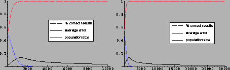
In the figures 8.6 to 8.8, I illustrate the learning curves obtained for each order of permutation, when the classifier population size allowed in the system is 100. The number of steps considered here are 15,000. The optimal problem description produces a function that can still be learned

  

Figure 8.3: Prediction results of permutation experiments (pop. 400).

  

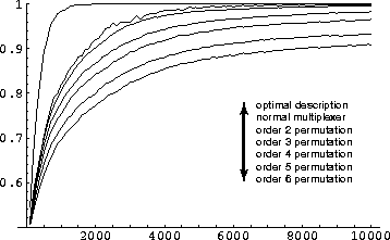Figure 8.4: Error results of permutation experiments (pop. 400).

  

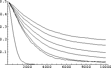Figure 8.5: Population results of permutation experiments (pop. 400).

  

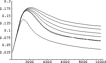Figure 8.6: Prediction results of permutation experiments (pop. 100).

  

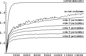Figure 8.7: Error results of permutation experiments (pop. 100).

  

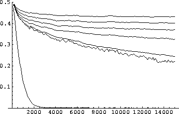Figure 8.8: Population results of permutation experiments (pop. 100).

perfectly by the system after about 3000 steps, allowing the population to be compressed to about 12 individual types. In the other experiment, one can see that having only 100 individuals in the population is problematic, although learning still occurs.

To explain this phenomenon, two reasons can be postulated. First of all, the classifier system cannot rely on a complete population of specific classifiers, this is a problem that will always occur in more complex experiments and must be coped with. The second reason is that although generalization would be possible, the system would need more working space to hold various classifiers as a genetic resource pool in addition to the accurate classifiers useful for action selection. We see for example that the number of different types of classifiers initially present in the system is around 50, that is, the genetic algorithm produces an average number of 50 different classifiers in a population of 100before the accuracy of these classifiers starts becoming differentiated. In the different permutation experiments, this variety is barely sufficient to differentiate the accuracies of the classifiers in order for the system to start eliminating classifiers. With the normal multiplexer problem and order two permutation problems, this compression of the population can engage and will eventually produce satisfactory results for learning the function, but with permutations of a higher order, the population compression stabilizes too fast for satisfactory learning of the function. Still it is remarkable that even in the case of completely random functions (order 6 permutations), the system is capable of making correct decisions 60% of the time on average.

Information Content

An optimal permutation that leaves the input information that is relevant to the classifier system in the rightmost bit is shown in table 8.2. Each one of the value bits that is addressed by a particular configuration of the first two bits is simply swapped with the rightmost bit (whatever its value). In this situation, the XCS can learn only the position of this bit and generalize away all the other bits, a situation for which I have plotted the learning curves on figure 8.10. One notices here that the number of steps until the system correctly predicts the choices that must be made is much shorter since the number of general classifiers that accurately describe the problem is reduced to a minimum of four. From the step 1500 onwards, the classifier system always makes the correct decision to maximize its reward and prediction error vanishes completely from step 2000 on. The diversity of classifiers in the population also reduces and stabilizes to 20 different types of classifiers after 15 thousand steps.

  

Figure 8.9: Results of the normal multiplexer: 10k and 30k steps.

  

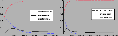Figure 8.10: Results of the optimal description problem: 10k and 30k steps.

The objection that might be raised by this example is that by finding an optimal description of the classifier inputs, one is in fact solving the problem for the system and that there is no point in further experimentation. This is precisely the point I am making, the compression of information in the inputs to provide the system with a description that is compatible with the functionality of the system is the missing feature of this system and this feature is also missing from most other adaptation algorithms that are used in AI. The regularities of the environment have to be written in the terms of an adaptation algorithm, here of the reward levels. In this problem, the environment that is the space of input strings in standard form has regularities that are not entirely detectable in terms of the classifier system. But to the system, there are only two important situations in the environment: those that provide a reward and those that don't. Usually, the complexity of an environment is much larger that what can be represented in a symbol system, but the situations that are important to the system can be expressed much more simply in the terms of that system. An algorithm that must deal with such environments should be able to extract this information itself in order to learn intelligent behaviors.

Experiment Parameters

The preceding results have been produced by generating a number of different test runs from random XCS system initializations. In the simple experiments, the standard description of the multiplexer problem and the optimal description of the multiplexer problem, 100 test runs were used to generate the averages plotted on the curves for correct results, error in prediction and populations. In the permutation experiments, 100 random permutations were generated for each order of permutation and in each case 20 runs of the XCS system were used to average the data, the overall averages are thus calculated from 2000 test runs.

The number of classifiers allowed in the system were respectively 400 and 50 for the two different sets of experiments. With four hundred individuals, the classifier system has sufficient resources to build a complete representation of the problem space with specific classifiers, although this will not usually happen since the classifier system is driven towards generalization by its internal mechanisms. With a population of 50 classifiers, the resources of the system are not sufficient to cover all the problem space and the system must be able to generalize in order to solve the problem.

The system parameters are the same as those given by Wilson in [70], with his more recent clarifications about implementation issues introduced: (available on the Internet at http://world.std.com/$\sim$sw/imp-notes.html)

• rewards distributed for correct or incorrect answers of the system are 1000 or 0 respectively
• the reinforcement parameters are: $\beta = 0.2$, $\gamma = 0.71$, $\varepsilon_0 = 10$, $\alpha = 0.1$, $\tau = 0.1$
• the genetic algorithm based parameters are: $\theta = 25$, $\mu = 0.04$, $\chi = 0.8$, $\delta = 0.1$, $P_{\char93 } = 0.33$
• initialization parameter for new classifiers were: strength = 10, error = 0, fitness = 0.01, experience = 0, covering experience = 0 and match set size estimation = 0

EMud Dynamic Test

Even though an XCS classifier system is seriously challenged when having to learn the dynamics in an environment, a simple experiment can be made, that shows the functional ability of the classifier system to adapt to an environment where the causal role of actions chosen is important. It was shown in the preceding experiment that the generalization capabilities of the XCS system depend largely on the coding of the information perceived, but that overall, the system is able to generalize in a satisfactory manner (at least when the information perceived is not too large). In this experiment, I want to show that assuming the perceptions of the environment can be generalized over, the system's ability to adapt to the dynamics of an environment is not influenced very much by the description of this environment.

The Switch Test

The experiment that I have used to show this is of learning a simple switch in the environment. Let me use the following informal terminology for the description of the problem, the system used in the experiment consists in:

• an agent: the (virtual) rat
• an agent: the cheesemaker
• a set of three connected rooms
• pieces of cheese
• rat ``traps''

In this system, the rat is the XCS agent that must learn to find and eat pieces of cheese. The three rooms are aligned with a western room, a central room and an eastern room each connected to its neighbor(s) by one exit. The cheese maker is an automatic agent that starts in the western room which is then empty. If the rat appears, he drops a piece of cheese and a ``trap'', moves to the east, drops a ``trap'' and moves to the east again, waiting in this eastern room until the rat appears. If the rat enters the room, he drops a piece of cheese and moves to the westernmost room, collecting the ``traps'' on his way. The cycle then starts over. In the experiment, the ``traps'' have no role other that to act as markers in the environment.

The rat agent must find a decision policy among four actions: moving east, moving west, eating cheese, being inactive for a turn. The sensory information he is provided with to make decisions consist in a string of five true/false statements: is there an exit to the west, is there an exit to the east, is there a trap here, is there a cheese maker here and is there cheese here. His goal is to accurately and generally associate each of the perception signals to one action. The perceptions thus form a space of 32 different possibilities and the possible classifiers in the system number 128. This problem, although simple, requires the system to break out of the typical looping behavior it is prone to enter when in a dynamic environment, indeed, a classifier system has the tendency to enter two step oscillations in such environments, since usually, one classifier starts having maximal prediction value and accuracy in one room, and then when moving to the next, another classifier will take over to bring it back to the first room, creating a regular two step pattern.

Here, the system must adapt internally to an optimal chain of more that two classifier choices, since the optimal behavior is to eat cheese if some is available, move west when no trap is present and a west exit exists or move east when an east exit is present and a trap is present. This forces a set of a minimum of three general classifiers to be found and maintained in the system. An XCS classifier system has no memory (in the sense of internal memory states), the way this problem must be learned by the system is through the multi-step reinforcement procedure of the algorithm. This multi-step reinforcement algorithm works by rewarding the classifiers that advocated an action on a preceding step with the immediate reward of that step and the discounted predictive value of the current situation. Here, reward was given for eating food and no other action was rewarded. The predictive value of moving or doing nothing is thus only derived from the probability of finding cheese and eating it on the next step, which leads to high levels of error value for the movement or inaction classifiers.

Result Plots

  

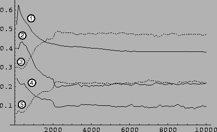
Figure 8.11: Results of the ``rat'' experiment (averages over 200 cases).

The results plotted here are those obtained by the situation described above, with the same parameter values as in the multiplexer problems. Since the goal of this experiment is not to find a perfect (but maybe unstable solution), no parameter adjustment was used, even though one can obtain almost perfect results by so doing. The result curves are plotted on figure 8.11, with the number of action cycles on the horizontal axis. Curve (1) is the normalized number of distinct types of classifiers in the XCS system, where a maximum population of 200 was allowed (.5means $200 \times .5 = 100$ classifier types). Curves (2) to (5) are then respectively the number of movements executed, the number of pieces of cheese eaten, the failed attempts to act and the inactive steps of the rat over the last hundred action cycles. In order to initialize the system with an exploration phase, a function is used to probabilistically allocate exploration and exploitation for each step. The function used has decreasing values between zero and one in the first two thousand steps and then stabilizes so that an average of one action cycle in twenty is an exploration cycle. In order to satisfy these criteria, the (somewhat arbitrary) function I have used is:

$$f(x) \stackrel{df}{=} \left\{ \begin{array}{ll} (\frac{x}{500... ...leq x < 2000$ } \\ .05 & \mbox{otherwise} \end{array} \right.$$

As can be seen on the graph 8.11, the population diversity in classifier types exhibits a similar behavior as in the multiplexer experiments, sharply rising at first and then reducing as accurate general classifiers are progressively found for the problem. This population stabilizes at around 80 distinct varieties of classifiers which is quite a large amount, given the maximum of 128 possibilities and the fact that only 4 should suffice to sum up the solution to the problem. The curves numbered (3) to (5) then represent the total actions of each type that the system uses to solve the problem (move, eat, do nothing). Since each action is equally likely to occur at the beginning of the experiment, there are about double the amount of moves as eat or ``noop'' actions. The initial differences reside in the fact that choosing to be inactive never fails, whereas choosing to eat will fail every time there is no food in the current locus. The last curve (4) is the number of failed attempts to do something, such as moving east when there is no east exit or eating when there is no food. Curves (2) to (5) sum up to 1 at each stage.

  

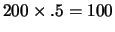
Figure 8.12: Results of the ``rat'' permutation experiments.

As illustrated, the system is able to find an equilibrium between the number of moves at each stage and the number of pieces of cheese eaten, the fact that the moves stabilize to about double the amount of pieces of cheese eaten indicate that the algorithm never oscillates between two neighbor locations, moving to the extremities of the environment at each passage. The failed attempts can then be accounted for by the fact that the agent then pushes on, trying to move further until the failed attempts (there is no east exit to move through in the eastern room) bring the predictive value of moving in that direction lower than that of moving in the other direction. Overall, this behavior is a good attempt at modeling the switching function of the problem, without the expressive ability to have a better approximation of the problem solution. With some changes in the parameters of the algorithm, it should be possible to minimize the failed attempts phase of this solution, but I have not investigated the matter in detail. The point that I want to make is that we can see here the way in which the classifier system attempts to express the dynamics of the environment within its own limited expressive capability.

Information in the Problem Dynamics

In the multiplexer experiments, the full information about the problem could be stored in terms of stable classifier predictions, with accuracy indicating whether a classifier was a good description of an environment regularity or not. Here, the information that must be acquired by the system is not static and each classifier does not have a definitive predictive value. Instead, predictive values will change over time for some classifiers, depending on the current situation of the agent: the full information for the problem resides in multiple step evaluations. For an XCS to capture this, it must still store the information in the classifiers, but most of this information is now held by the prediction, error and accuracy values of these classifiers, since the predictions now have a continuous range of possible values that dynamically vary from situation to situation. The characterization of the system's functionality now depends much less on its ability to generalize over the input perceptions of the system, than on its ability to express the dynamics of the problem in the predictive values of the classifiers.

To highlight this, I have reproduced the same experiment, but with other perceptual descriptions of the environment. As in the multiplexer problems, I have coded the perceptual inputs from the environment by using random permutations of the input space. When this is done, the XCS system must generalize its representation of the world in terms of classifiers, but without the same regularities in the inputs. The data for these experiments (averaged over 200 sample random permutations) show that although the diversity of classifiers in the population is affected (it increases), the solution to the problem that is found by the algorithm gives the same results. The global results are shown on figure 8.12, while the comparative results are shown on figures 8.13 and 8.14.

  

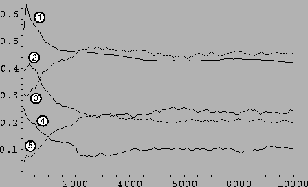
Figure 8.13: Comparative results, moves and eating.

  

Figure 8.14: Comparative results, population, failed actions and ``noops''.

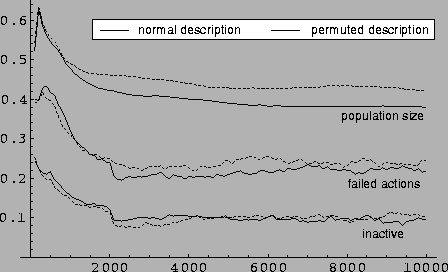Clearly, the perception of the environment affects the classifier system in its operation, but this effect is limited to the representational ability of the system and not the way in which it can learn the dynamics of the environment.

Discussion

The two experiments described in this chapter show that information compression (in the sense of generalization for a classifier system) is an essential feature of an agent algorithm that must learn in rich environments. Every algorithm developed in the field of AI for such agents is capable of some form of generalization, be it implicit or explicit. What differs from system to system is the internal structure and functions in which this information compression is expressed. It is this language of representation that characterizes an algorithm. As we have seen in the preceding experiments, there is a range of problems that can naturally be addressed by a classifier system, and others that simply are not adapted to such systems. This expressivity factor is fundamental when choosing an algorithm to solve a problem and is already intuitively understood by most scientists, but has not been formalized as I find necessary: when attempting to solve real world problems, a connectionist approach is often chosen for its ``continuity'' properties and when a modern expert system is implemented a symbolic approach is preferred, but no precise characterization of the relevant properties of each system has been attempted. Since every problem has a distinct type of regularities that must be integrated by agents programmed to solve them, I would like to propose that it is now time for AI researchers to focus on a classification of algorithms, based on their generalization capabilities and internal dynamics.